The Friday Gold Trade: A Conditional Edge
Seventeen years of Friday closes — and two-thirds of them are noise.

Gold drifts higher on Fridays. The effect is statistically significant, it has persisted for decades, and most traders who know about it trade it unconditionally. The useful question is not whether this is true but under which market conditions it is true — and the answer changes everything about how you trade it. This article builds a hypothesis about the mechanism behind the Friday effect, derives a filter from that hypothesis, and shows that two-thirds of all Fridays are noise while the remaining third is where the edge actually lives.
Gold Has a Friday
The starting point is a simple empirical observation. Take daily returns for gold and equities and sort them by weekday. Most of what you find is noise. But two bars stand out.
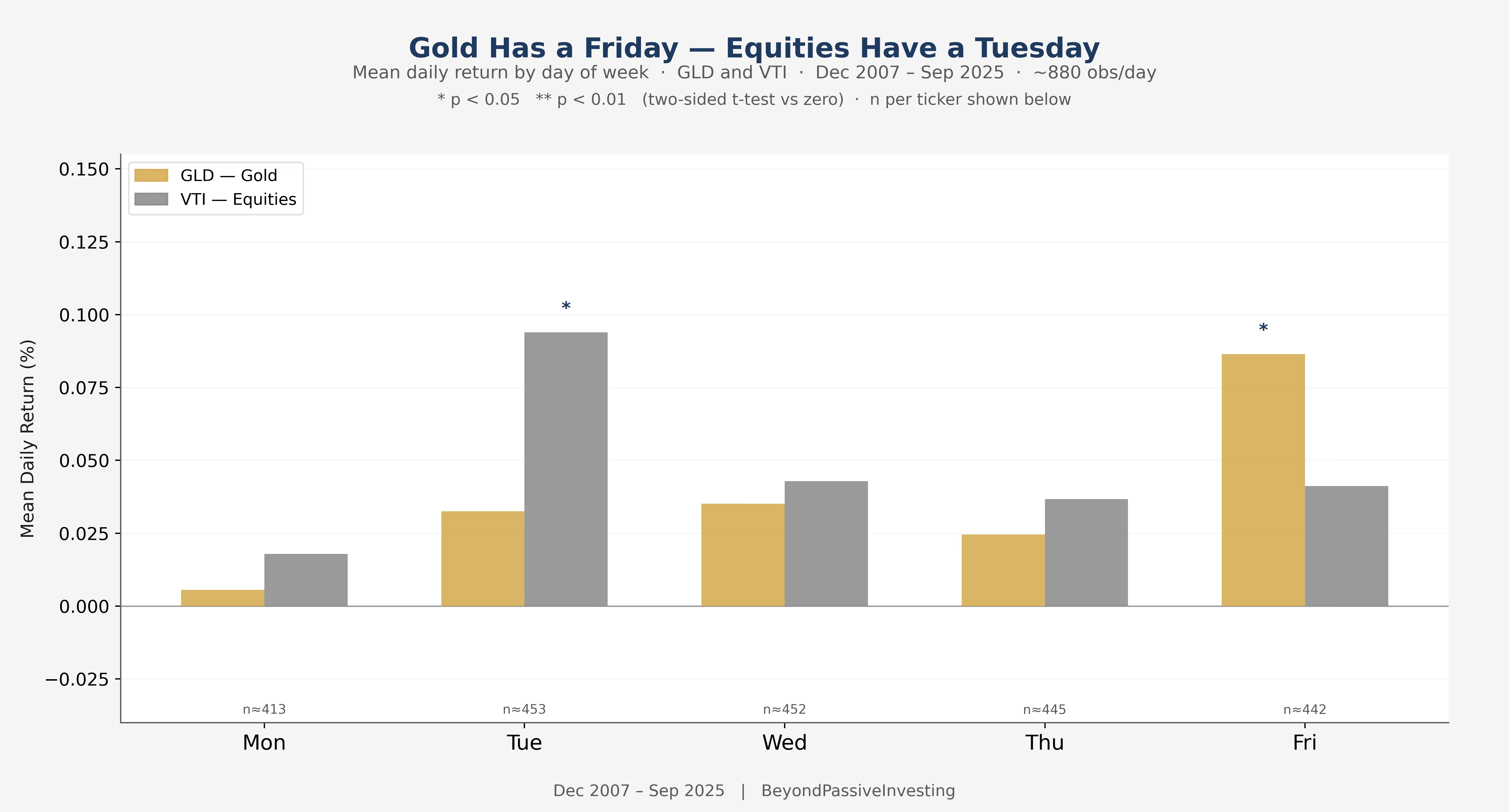
Gold drifts upward on Fridays. Equities drift upward on Tuesdays. With ten combinations to test across five weekdays and two assets, one false positive would be expected by chance at the 5% level — so the pattern alone proves nothing. What matters is whether there is a structural reason for these specific anomalies. For Friday gold, there is, and it is simple enough to state in a sentence: institutional risk managers need to sleep on weekends.
Options desks delta-hedge into Friday close. Risk managers reduce gross exposure before two days during which they cannot react to breaking news. Institutional hedgers add tail-risk protection when positions cannot be monitored. This demand is predictable because the calendar is predictable, and it concentrates in assets that are liquid, globally recognised as safe havens, and cheap to trade quickly. Gold is the most liquid safe-haven instrument in the world — the natural destination for precautionary weekend positioning.
A De-Risking Trade — But Not Always
If the Friday premium is a de-risking flow, it should not be constant across all market conditions. When markets are perfectly calm, there is little to de-risk against. Conversely, when markets are in outright crisis, the trade has already been on for days. Panic positioning is not systematic — it is desperate, and it plays out at whatever price clears the market, not through the orderly Thursday-afternoon flow we are trying to capture.
The interesting regime is in between: sustained, elevated but non-catastrophic anxiety, where risk managers are actively thinking about weekend exposure but where the situation has not tipped into forced deleveraging. If this hypothesis is correct, sorting Fridays by the prevailing level of market stress should reveal that the premium is concentrated in that intermediate zone and fades at both extremes.
The question is how to measure it. Absolute VIX level is an obvious candidate, but it conflates two different things: the level of fear and the direction of fear. A VIX of 22 that has been falling for three weeks is a different environment from a VIX of 18 that has been rising for a month. What we want is not the absolute level of implied volatility but whether the market is pricing near-term uncertainty above or below its medium-term baseline — whether fear is building or dissipating. The ratio of short-term to three-month implied volatility captures exactly this.
The Term Structure of Fear
The VIX/VIX3M ratio compares short-term to three-month implied volatility. In calm markets the term structure is in contango: VIX3M exceeds VIX, short-dated options are cheap relative to longer-dated ones, and the ratio sits well below 1.0. As fear builds, short-dated volatility rises faster than three-month, compressing the ratio toward parity. When the ratio crosses 1.0 — outright backwardation — the market is pricing immediate risk above its medium-term baseline: the signature of genuine crisis.
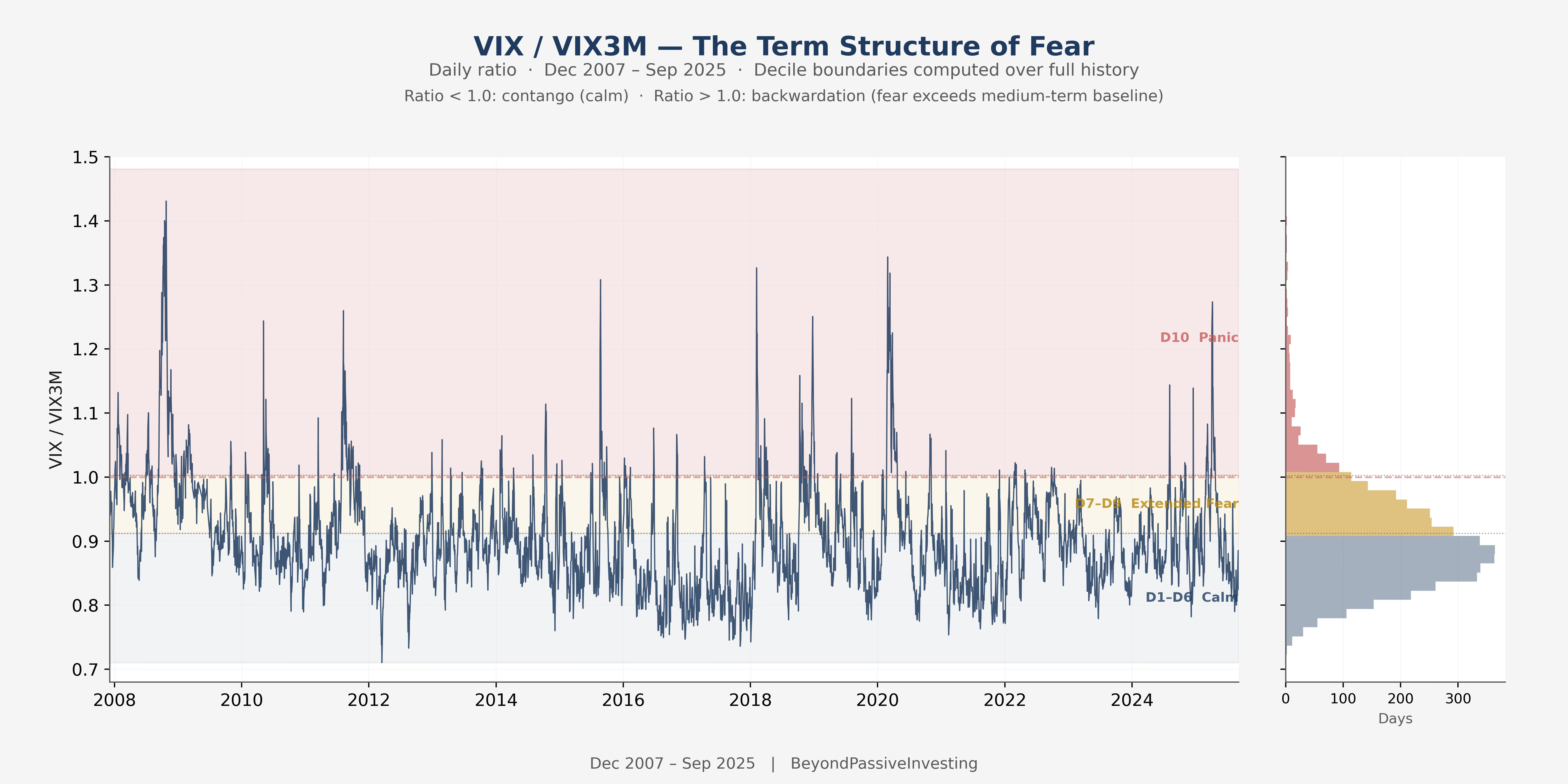
The chart divides 4,430 trading days into ten equal buckets by this ratio. Deciles 1 through 6 are the calm regime. Deciles 7 through 9 — the extended fear zone, ratio between 0.91 and 1.00 — are where the de-risking hypothesis predicts the Friday premium should be concentrated. Decile 10 is outright backwardation: the market expects things to be worse immediately than three months from now, the signature of episodes like the 2008 financial crisis, the 2020 pandemic shock, and the 2022 rate cycle.
If the de-risking hypothesis is correct, the Friday gold premium should be strongest in deciles 7 through 9 and should fade in both the calm zone and in full panic.
The Flow — and Its Monday Unwind
Sorting Friday gold returns by Thursday’s VIX/VIX3M decile confirms the hypothesis cleanly. One methodological note: the Monday panel could in principle use Friday’s decile reading, since Monday follows Friday. We use Thursday’s reading for both panels. The VIX/VIX3M ratio on Thursday is what triggers the trade — it is the observation that drives the entry decision. Using the same Thursday reading throughout treats the full Thursday-to-Monday arc as a single event conditioned on one fear state.
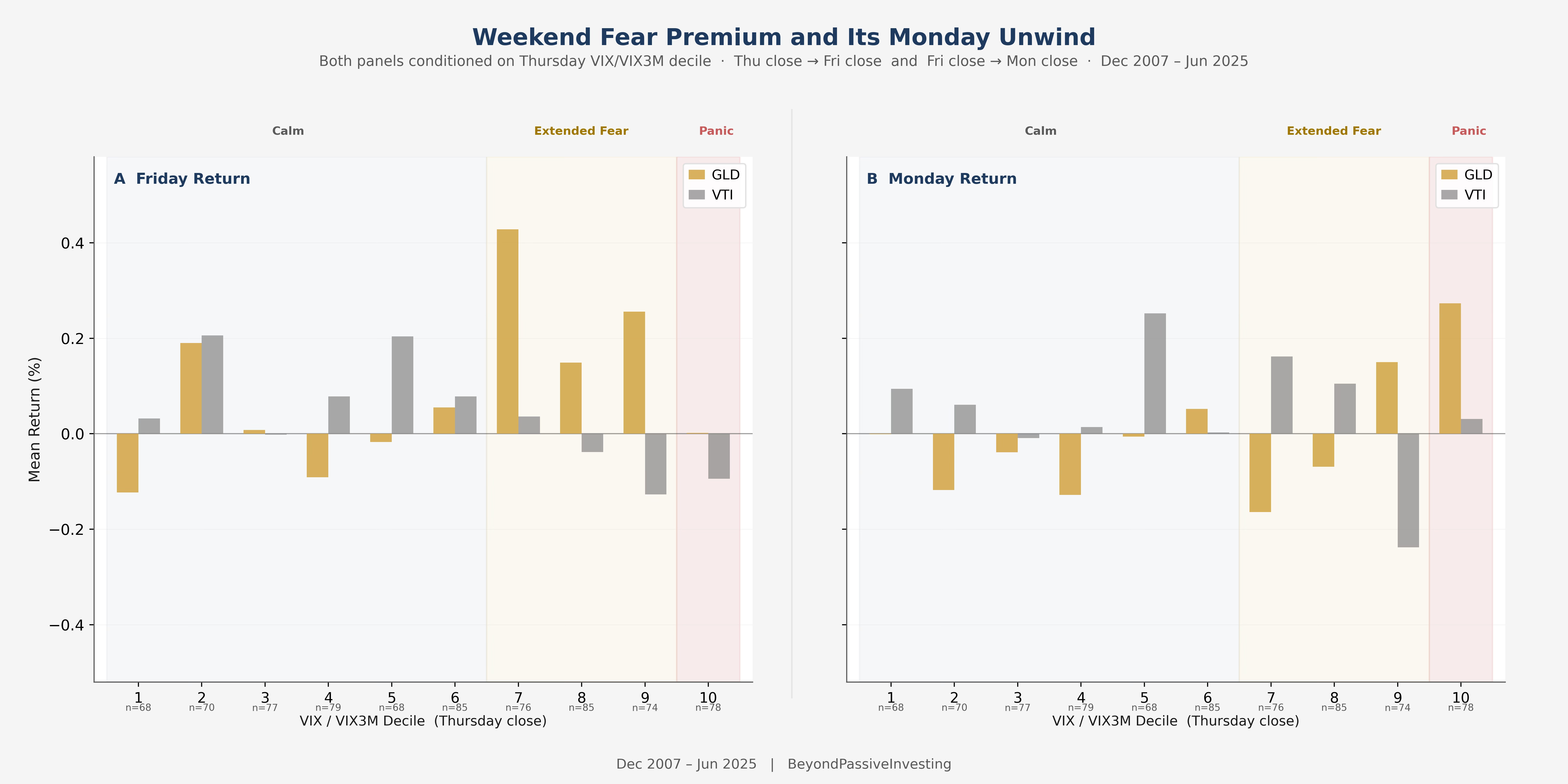
In deciles 7 through 9, gold averages between +0.15% and +0.43% on Friday. Equities are flat to marginally negative — not sold, simply not bid. The flow is additional hedging capacity being deployed on top of existing positions. The Monday panel confirms the mechanism. In deciles 7 and 8, equities bounce and gold gives back a portion of its gains. The precautionary hedge purchased Thursday afternoon is sold Monday morning after an uneventful weekend. Decile 10 tells the opposite story: gold holds its bid into Monday because in full backwardation the fear was not precautionary — it was a correct near-term assessment that continued to resolve into the new week.
From Noise to Edge — Reading the Statistical Evidence
Before building a strategy around any pattern, it is worth asking what the statistical evidence actually says. The t-statistic is the right tool: the ratio of the observed mean to its standard error, where the standard error equals the standard deviation divided by the square root of the number of observations. A t-statistic above roughly 2.0 — p-value below 5% — means the observed mean is unlikely to have arisen by chance if the true edge is zero.
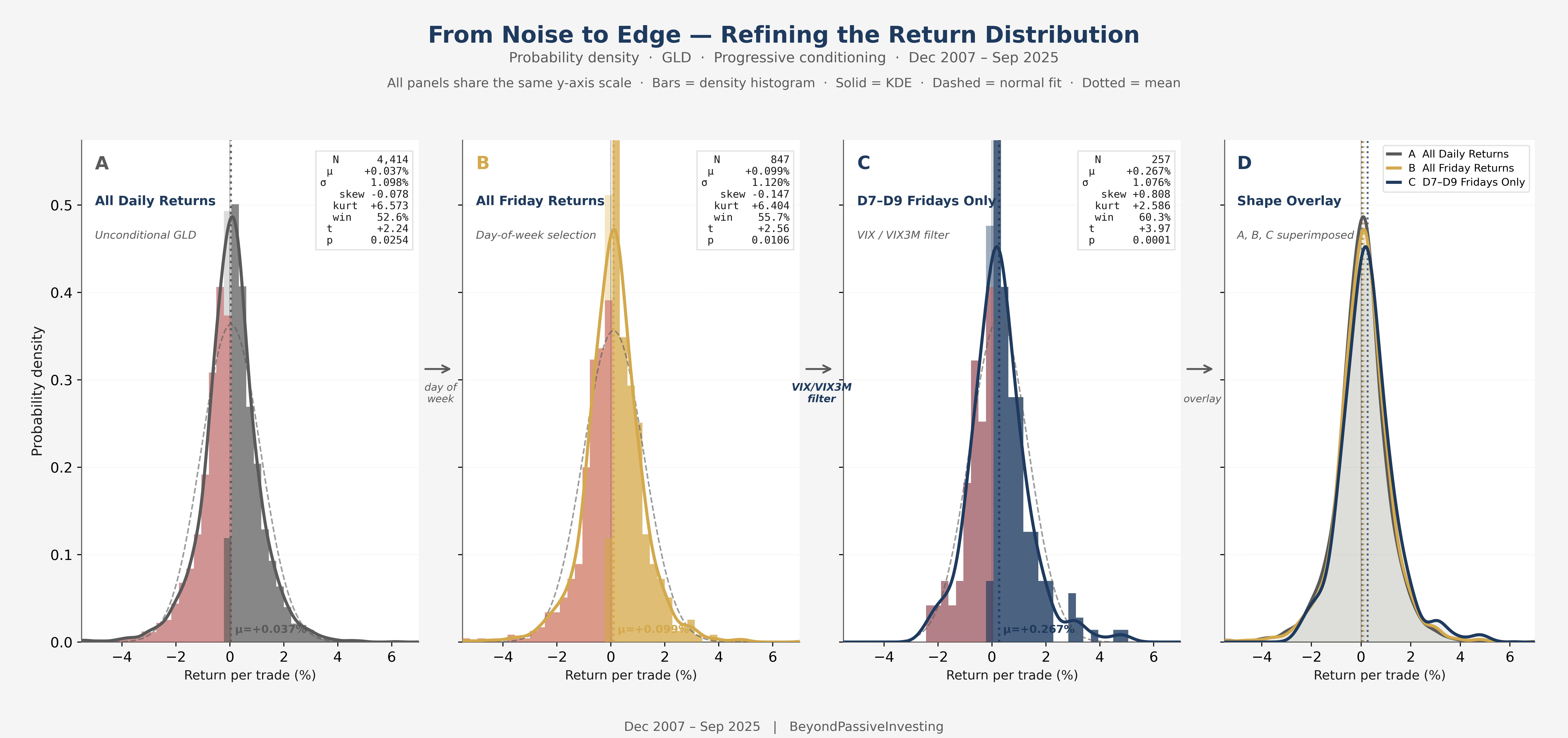
The unconditional daily gold return in this sample is +0.037%, against a standard deviation of 1.10%. The noise is thirty times the signal per observation. Accumulating enough data to achieve a t-statistic of 2.0 from this base requires approximately 3,500 daily returns — about fourteen years. The edge is real but utterly invisible at the trade level and takes over a decade to establish statistically from daily data alone.
Selecting only Fridays triples the mean to +0.099% while leaving the standard deviation essentially unchanged at 1.12%. The noise has not shrunk — the signal has grown because Fridays systematically overrepresent the hedging sessions. You now need 516 observations to reach the same confidence: about ten years of Fridays. Filtering to deciles 7 through 9 pushes the mean to +0.267%. The required sample drops to 65 trades — a threshold this strategy crosses in under five years of live trading. You can validate the edge from your own forward data before the end of the decade.
The distribution panels reveal something beyond the numbers. The standard deviation across all three series is nearly identical — the width of the distributions does not change. What changes is first the mean, and then in panel C the shape itself. The unfiltered distributions carry negative skewness and excess kurtosis above 6.0. The filtered distribution has skewness of +0.81 and kurtosis of 2.6. The left tail is truncated. The worst trade is −2.4% rather than −7.4%. The filter does not find a quieter subset of returns. It finds a differently shaped one — tilted toward wins by a mechanism that is structural rather than accidental.
The Equity Record
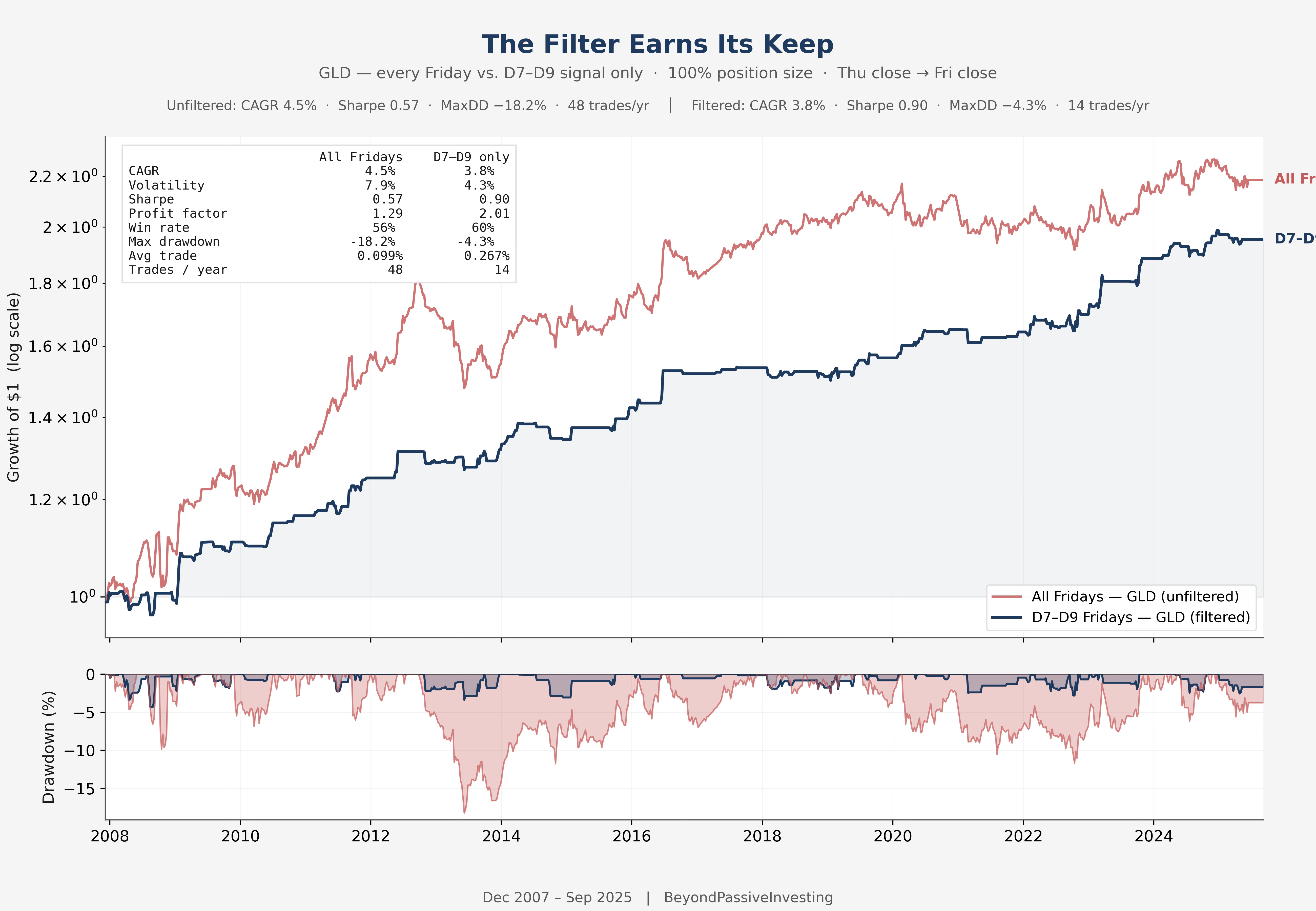
The unfiltered strategy — buying gold every Thursday since December 2007 — produces positive compounding and a Sharpe of 0.57. That is not bad in absolute terms, but it is noisy: drawdowns to −18%, a profit factor of 1.29, and an average trade of +0.10% against 1.12% standard deviation. The filter raises the average trade to +0.27% while the standard deviation barely moves. Sharpe rises from 0.57 to 0.90. Maximum drawdown falls from 18% to 4%. Every improvement traces directly to removing sessions where the institutional de-risking mechanism is not operating.
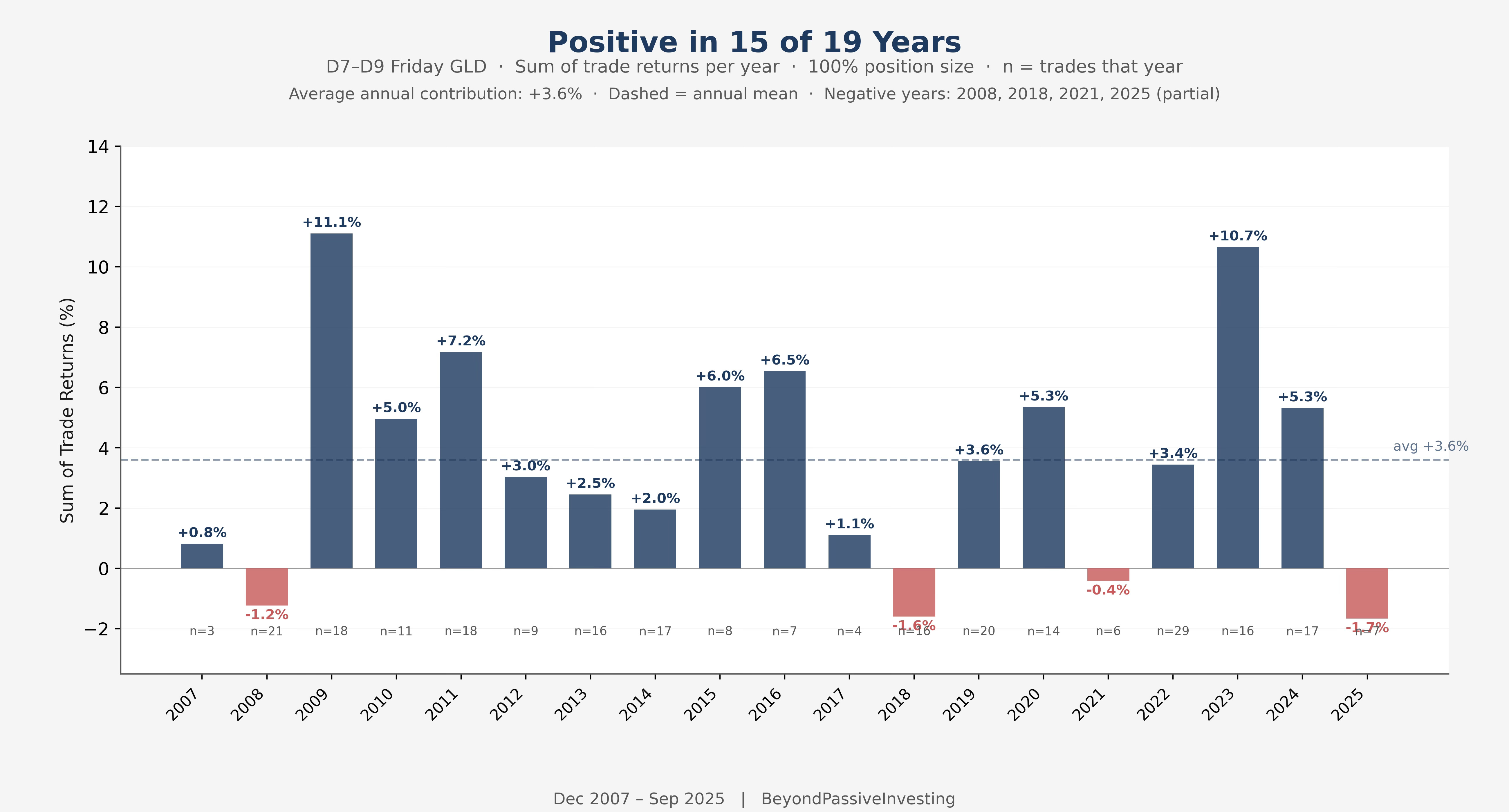
The annual breakdown shows 15 profitable years out of 18, including all three major stress episodes in the sample. The strategy earns in structurally different environments — post-crisis anxiety in 2009, the China flash crash in 2015, the pandemic in 2020, the rate shock in 2022 — because in each case the common feature is sustained VIX term structure compression without full-scale panic. It works when fear is a chronic condition rather than an acute one, which is exactly the environment the mechanism predicts.
Sizing and Implementation
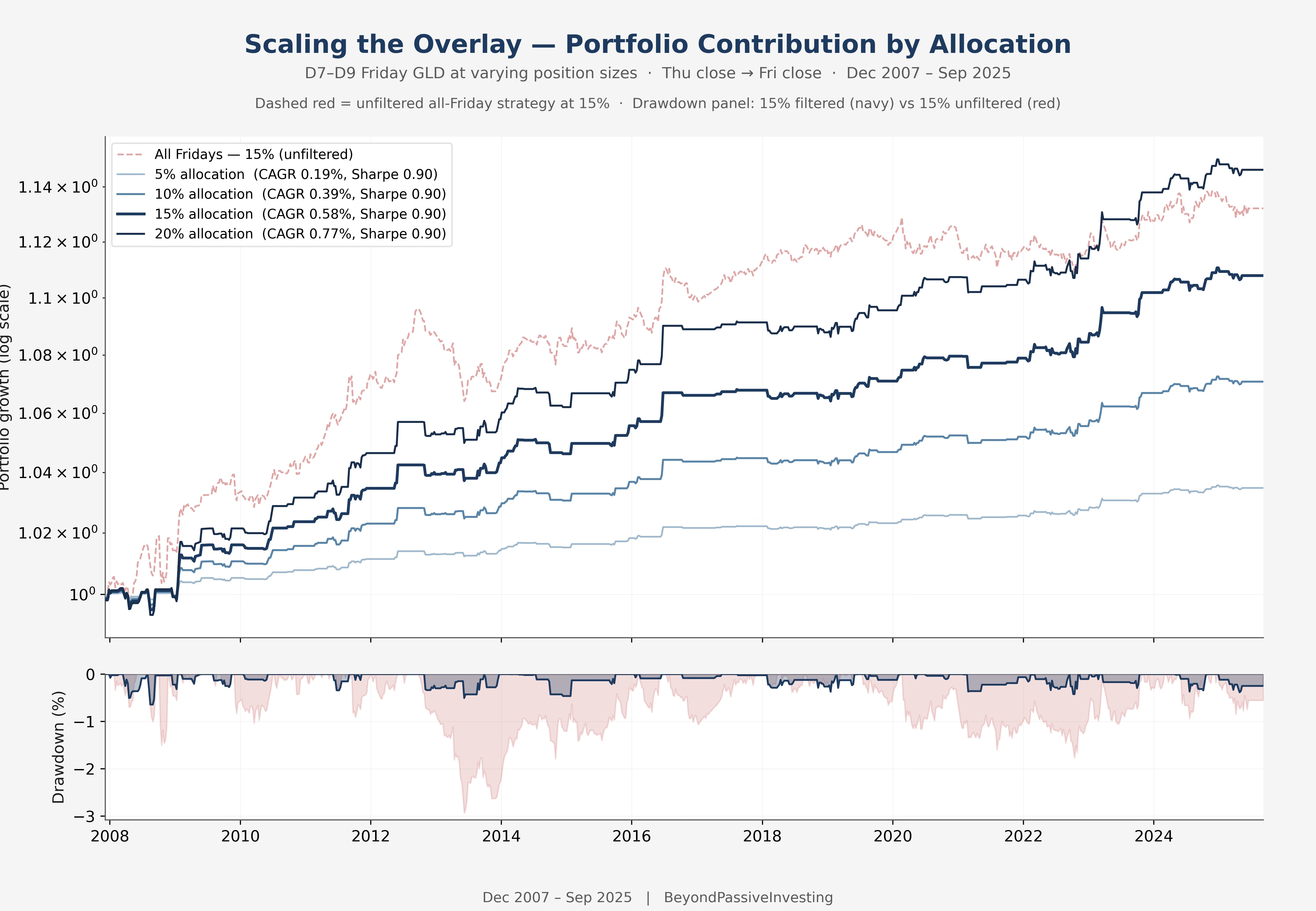
At 100% position size the numbers are illustrative. The correct framing is as an overlay on a base portfolio — the strategy is in cash roughly 94% of the time — 15 one-day trades out of 252 annual trading days — and can coexist with any longer-term allocation without competing for capital. At 15% allocation, the strategy adds 0.58% to annual CAGR with a maximum portfolio drawdown of 0.64%. The Sharpe of the overlay remains 0.90 regardless of allocation chosen, since return and volatility scale together.
For ETF implementation using market-on-close orders, the backtest carries a small look-ahead bias: the VIX/VIX3M ratio is observed at the Thursday close, which is the same moment as the assumed entry price. In practice, the MOC order is submitted before the close, meaning the signal and the fill price are determined in the same auction. The resulting bid-ask spread in GLD — typically one to two cents on a $240 ETF, roughly one basis point — is economically negligible assuming automated execution. The CME micro gold futures contract is equally cost-effective for this purpose.
Beyond the Friday Close
The temptation with a result like this is to keep refining: a tighter decile range, an additional absolute VIX filter, a momentum screen layered on top. The distribution analysis argues against it. The current filter already captures the mechanism almost completely. What remains outside D7–D9 is noise, and optimising for noise produces strategies that look better in backtests and worse in production. A Sharpe of 0.90 on 15 trades per year is a clean, robust result. At this trade frequency, each additional parameter consumes years of statistical power.
The more productive direction is horizontal: combining non-overlapping event trades within the same capital allocation. A 15% position here is in cash roughly 94% of the time — that capital is available for other systematic trades on other days without any overlap.
The day-of-week chart at the top of this article contains one more statistically significant bar. Equities on Tuesday. Same significance level, opposite mechanism — not the anticipation of weekend fear, but its resolution. That is the next article
.
Complexity explained simply. Very nice article and methodological
very nice and simple strategy, might try it out