
Trend following (1/4): Replicating your own program

The published literature on trend-following replication treats the program being copied as a black box. When the program is your own, this is the wrong way around — and fixing it changes the result more than I expected.
The story of trend following as a systematic strategy reaches back to the 1970s, when a handful of futures traders observed that prices in commodity markets tended to persist in their direction, and that a simple rule for following that persistence worked across very different markets and decades. The academic literature caught up later, in Moskowitz, Ooi, and Pedersen (2012) and the century-long study of Hurst, Ooi, and Pedersen (2017). By then the major funds — Man AHL, Winton, Lynx, Aspect — had been running the strategy for thirty years.
The result is unusual in finance: a positive-Sharpe strategy that survived publication, holds across asset classes, runs low-correlated to the equity premium, and has been visible for forty years. For a private brokerage account, the question is access. The published versions run with fifty to a hundred futures markets, prime brokerage, margin desks. The strategy works. Getting at it from the outside is the problem.
The standard answer is the CTA-clone product — SG-Trend Index ETFs, DBMF, others. The construction is the same in each case: take the index’s published return series, regress it on a small set of liquid contracts, trade the regression weights. The replica works, after a fashion. Something is being given up, though, and noticing what gets given up suggests a better approach when the program being replicated is your own.
What follows walks through that. The first half specifies the program — signal design, volatility normalization, universe. The second half shows why the standard clone falls short and proposes the alternative. The bottom-up versus top-down framing aligns with Butler, Gordillo, and Philbrick (2023).
What we are trying to copy
The strategy is straightforward in structure. The signal design is conservative on purpose — the project is to replicate a program with known intended weights, not to invent a better signal — and is held fixed throughout the series (Clenow 2013, Carver 2023).
The per-contract signal is the standard averaged-momentum z-score, computed across four lookback windows spanning the conventional short-, medium-, and long-trend horizons. For each contract on each trading day, we compute four price-change z-scores, average them, and clip the result. The clip prevents any single contract from accumulating an enormous position when prices have moved far. This is the workhorse construction of every diversified CTA program.
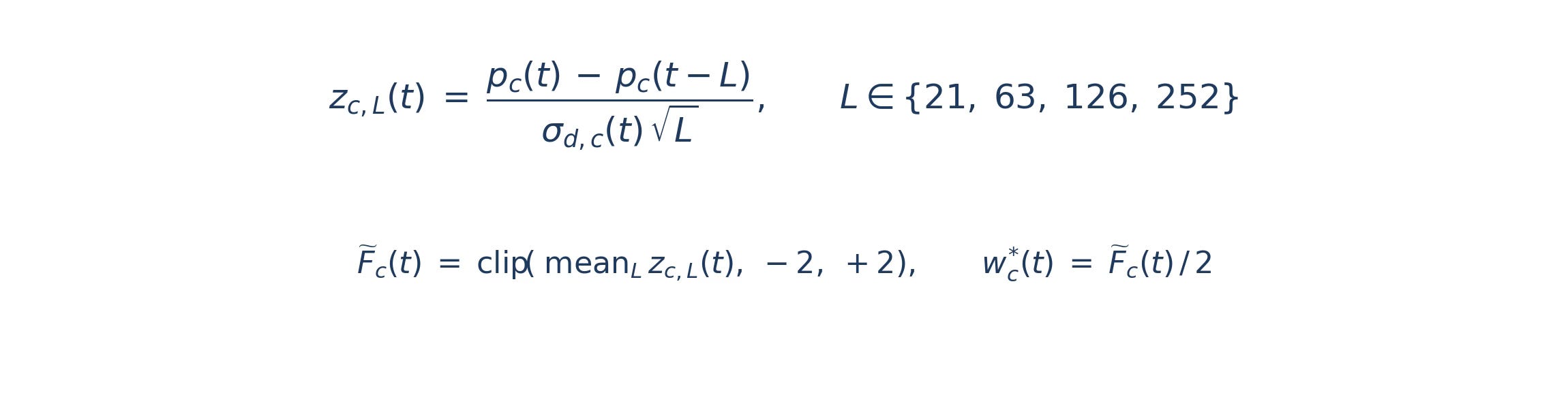
The volatility estimate in the denominator is the trailing 63-day standard deviation of the contract’s daily price changes — about a quarter of a year. The same estimator runs in the EUR/USD hedging work that combined carry and trend signals into a single overlay. Using a consistent vol window across applications makes signals comparable when components are combined later.
Volatility normalization happens at two levels, and the order matters. Each contract’s position is sized so one unit of forecast corresponds to one unit of risk. Contracts are aggregated within their CFTC sector, the sector basket rescaled to four percent annualized volatility using its own 63-day realized vol, and the ten sector baskets summed into a portfolio rescaled to ten percent. A single portfolio-level rescaling would let energy noise dominate during commodity vol spikes. The choice to normalize by CFTC sector — rather than by some discovered grouping — is itself a design decision, revisited in Part 2.
The cadence is once per week, applied after settlement in each contract’s home market. Futures settle at different exchange-local times, so “weekly rebalance” means “after this week’s prices are final everywhere.” Weekly is the compromise between daily — marginally higher Sharpe at much higher turnover — and monthly, which loses too much signal stability.
The universe is the 62 most liquid futures contracts spanning equities, fixed income, currencies, energy, metals, grains, soft commodities, livestock, and cryptocurrencies.
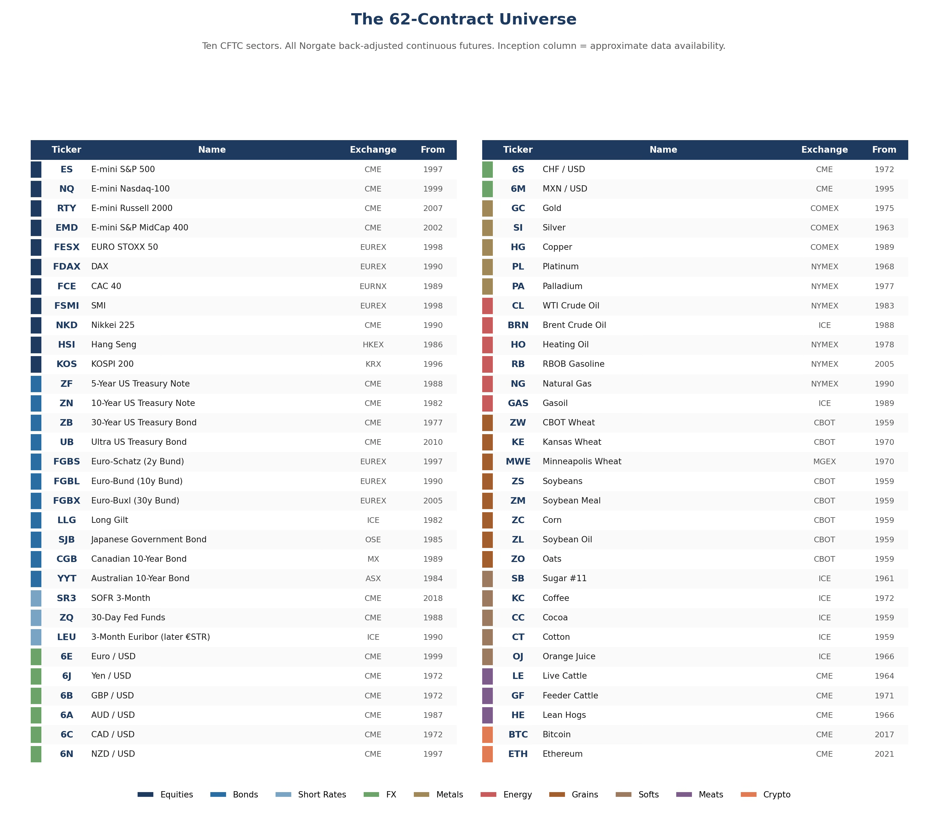
The composition reflects accessibility and data history rather than economic theory. CME and EUREX dominate the financials because their contracts have the deepest data; metals and energy split across COMEX, NYMEX, and ICE; the soft commodities live almost entirely on ICE. The cryptocurrency contracts are included despite short histories — excluding them on duration alone would be motivated reasoning given how much trend signal they have actually provided since 2020.
Price data comes from Norgate Data, which provides per-contract OHLCV histories and pre-built continuous series for each market. The continuous series are arithmetically back-adjusted (point-based): at each roll date, the historical portion is shifted by the price difference between the new front-month contract and the expiring one, so the splice produces no artificial gap. Norgate rolls cash-settled contracts on the business day before final trading and deliverables on the business day before First Notice Day. The Close field is the official exchange settlement price rather than the last-trade print — which matters for any vol-normalization built on daily returns, since settlement prices are what margin and risk calculations clear against.
One execution detail worth flagging. The live system applies a per-contract notional cap of five times NAV, to protect against pinned-rate regimes where short-rate contracts (SR3, ZQ, LEU) would otherwise demand huge notional exposures relative to their near-zero realized volatility. The baseline backtest does not enforce this cap; the impact on aggregate Sharpe is negligible because the cap binds only on these specific contracts in specific regimes, but a live implementation needs the guard.
The baseline
Running the construction described above on the 62-market universe from 1995 through April 2026 produces the equity curve below.
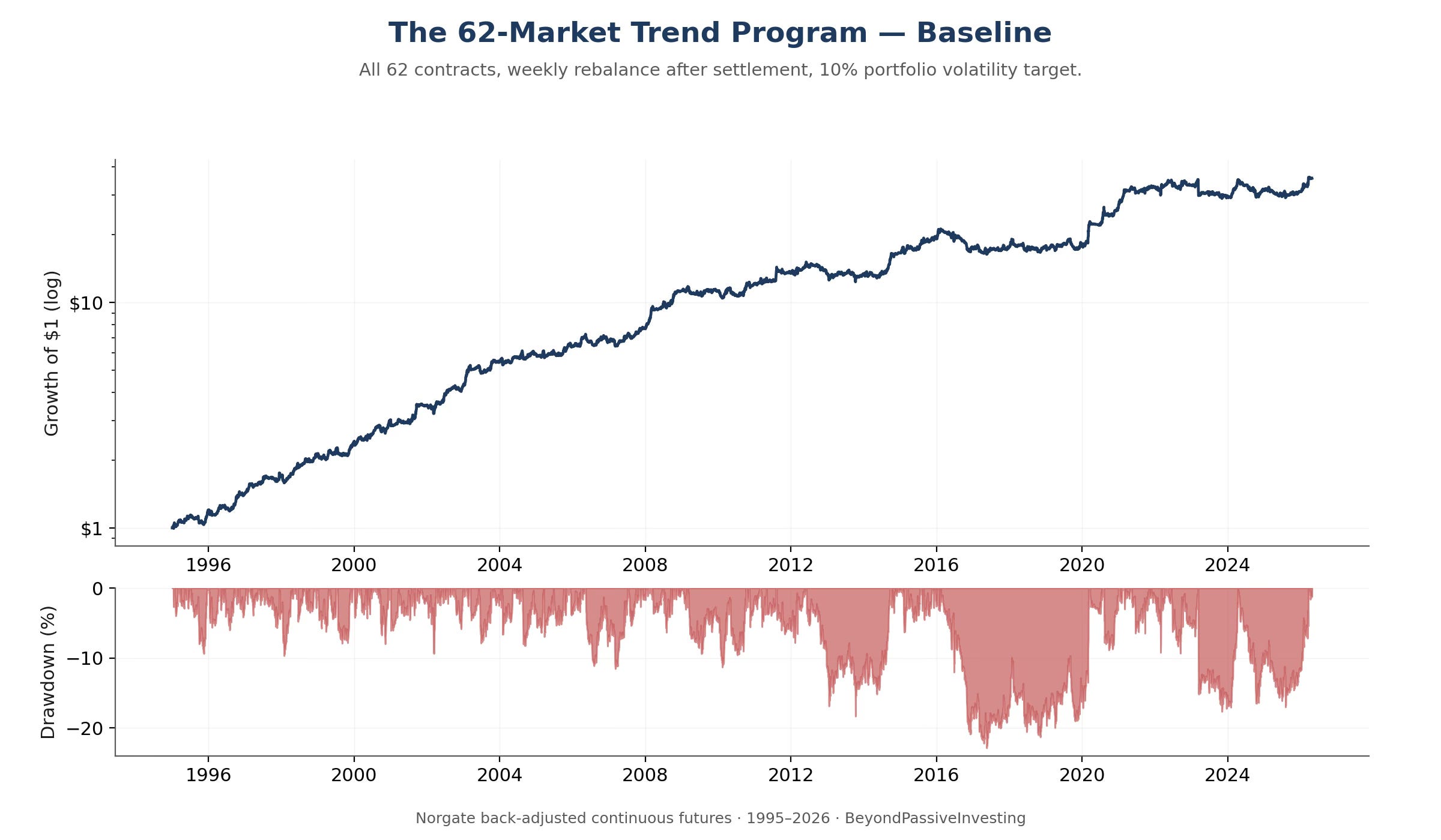
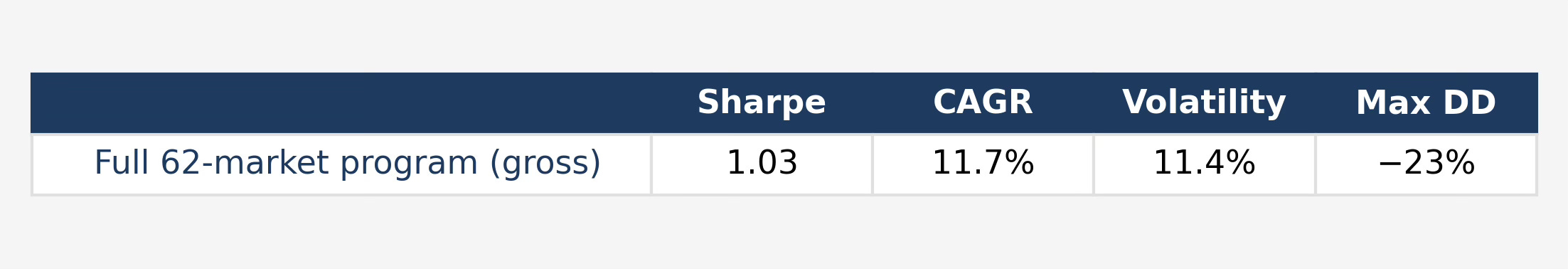
The Sharpe of 1.03 is gross of transaction costs. A continuous-trend program of this kind turns over roughly six to ten times per year, with one-way slippage of two to three basis points across the universe — lower for index futures and US Treasuries, higher for thinner softs and metals. That translates to 30 to 50 basis points of drag per year, a Sharpe deduction of 0.03 to 0.04. The net number an actual implementation would deliver is around 1.00 — consistent with the SG-Trend Index’s published track record over the same window.
This is honest for a thirty-year out-of-sample run. The 1980s and 1990s — the trend-following golden era — ran considerably higher in this universe, around 2.1 over the 1990s alone. Pulling the start date to 1995 removes the strongest tailwinds. Older trend-following literature quoting Sharpes in the high ones or low twos typically uses samples that include those regimes.
Trading the program as constructed requires positions in all 62 markets, capital to support each, and operational machinery for quarterly rolls and weekly rebalancing. The retail-replication question is how to compress this without losing the program’s behaviour.
Three regressions
The standard approach to compressing a trend program is borrowed directly from index replication. Regress the program’s published return on a candidate set of liquid contracts, take the regression weights, trade them. This is how every public CTA-clone product is built — Butler, Gordillo, and Philbrick (2023) survey the literature. The replica works, after a fashion. But the construction makes two compromises that are not load-bearing, and unwinding them changes the result.
First compromise: the weights. The elastic-net regression chooses both which contracts to use and what weights to assign them. The weights are the values minimizing squared error against the target over the fitting window. In a classical inverse problem — the kind I encountered during my physics PhD — those weights would be the principled estimate; the math says use them. Finance does not have those properties. The target rotates every month. The covariance structure is not stationary across decades. The regression weights overfit the in-sample window and drift out of sample; the contracts they pick are sensible, but the loadings they assign are not. Trading the selected contracts at equal weights keeps what the regression delivers reliably (the selection) and discards what it cannot (the precise loadings). The literature on this is older than the CTA-clone problem: Michaud (1989) on optimization error, DeMiguel, Garlappi, and Uppal (2009) on the 1/N portfolio.
Second compromise: the target. The realized return of any trend program is a heavily compressed summary. Each day the program held positions in dozens of markets, each with its own size and direction, and the daily return collapses all of that into a single scalar. Regressing contract returns on that scalar asks the regression to recover behaviour from a one-dimensional projection of it. The recovery is necessarily approximate, and lagged: the replica drifts behind regime changes rather than tracking them. But — and this is the move — when the program being replicated is your own, you observe something the external replicator never sees. The program’s current state, the 62-vector of target weights it intends to hold this month, is sitting in front of you. The state is uncompressed; the history is compressed. Working with the state rather than the history is the conceptual shift; everything else is mechanics.
The construction. Take this month’s target weight vector. Project it backward across a 504-day trailing window: for each historical day, compute the return the program would have earned if it had held the current weights continuously. This is a counterfactual — past months actually used different weights — and that is the point. We are not asking about the program’s true history. We are asking what the current allocation behaves like, and the question is best answered by holding the allocation fixed. The resulting series is the synthetic backtrack:

The elastic net is asked to find a sparse weighting of the universe whose own combined trend stream best approximates this synthetic series:

The L1 term drives sparsity; raising α with ρ = 1 zeroes coefficients out one at a time. The L2 term drives shrinkage; it pulls all coefficients toward zero, stabilizing the solution when contracts are correlated. Mixing them at ρ = 0.5 gets both: a sparse selection that is also stable across refits. Getting exactly ten contracts is a matter of binary search on α — start wide, fit, count nonzeros, adjust. The selected contracts are then traded exactly as they were inside the full program: each on its own trend forecast — the same per-contract momentum signal, normalized by that contract's own volatility — so that a flat or fading trend in any one contract shrinks its position toward zero automatically. This is the sense in which the weights are equal: not equal dollar exposure, but equal risk per contract, with direction and conviction supplied by each contract's individual signal rather than by the regression. The regression chose which contracts; the trend forecasts, computed once for the whole program and simply reused, decide how much of each to hold. The combined book is then vol-targeted to the same ten percent used in the full program. Positions rebalance weekly with the signals; the contract selection refits monthly.
The result
Applying this construction — synthetic-backtrack target, ten selected contracts at equal weights, monthly refit — produces the curve below, alongside the realized-return clone for comparison and the full 62-market program in light gray as a reference.
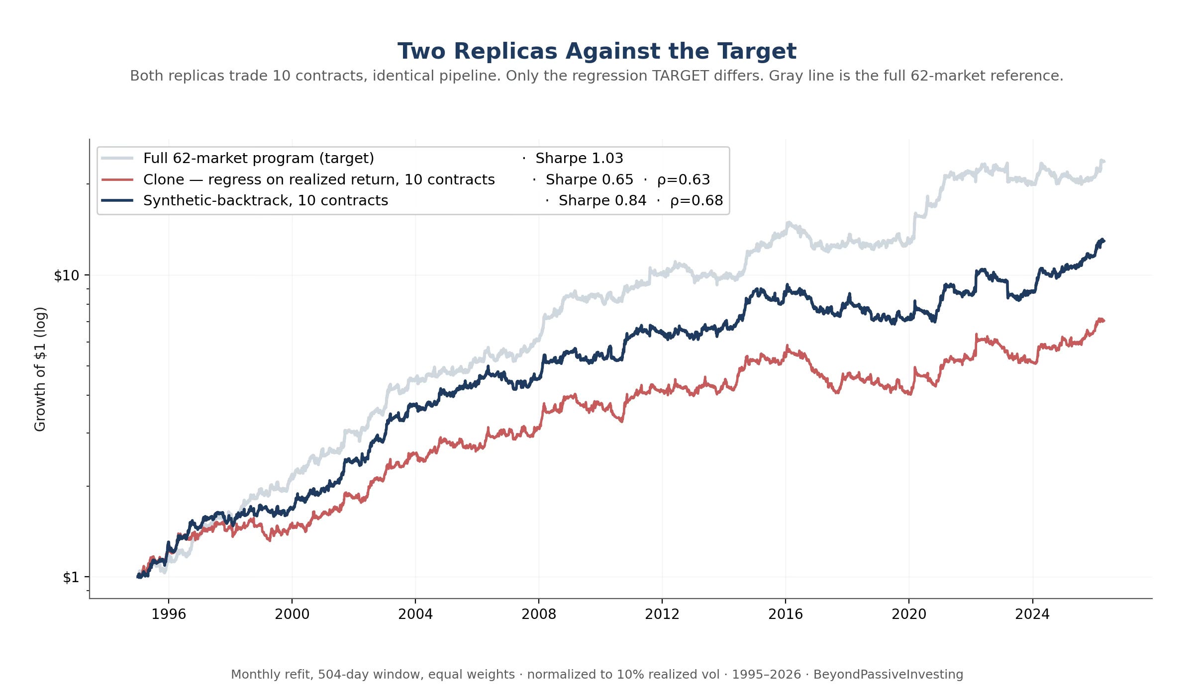
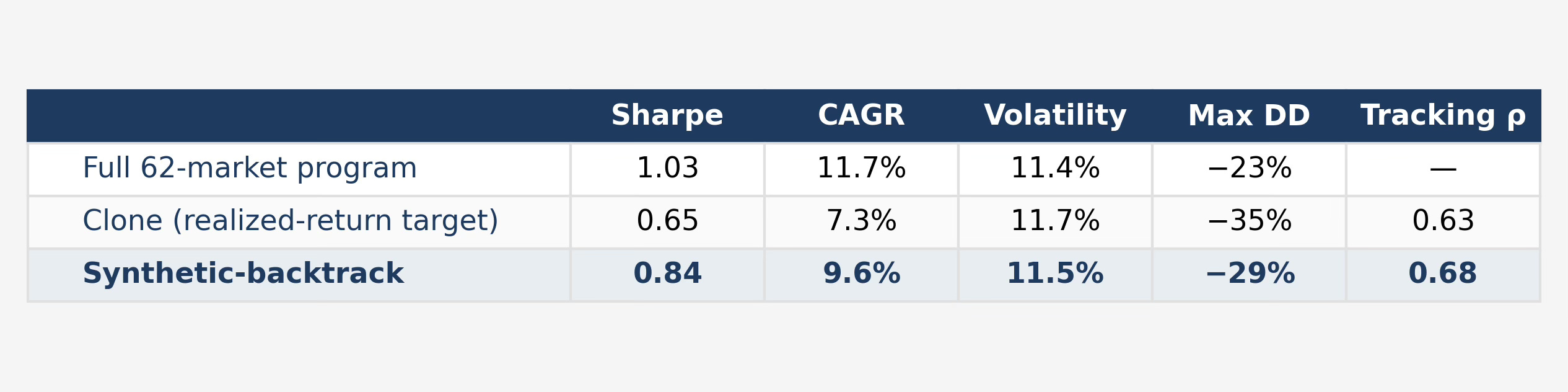
The synthetic-backtrack runs at Sharpe 0.84 against the clone’s 0.65 — an improvement of 0.19 over the thirty-year window from a single change to the regression target. Tracking correlation rises with it, from 0.63 to 0.68. Both quantities moving together is the right kind of result: when Sharpe rises while replication correlation falls, the regression has drifted into Sharpe-chasing; here the replica is genuinely closer to the target while also earning more. The equal-weights choice is borne out by direct test: same pipeline with regression weights yields Sharpe 0.88 but tracking correlation 0.17 — a fund, not a replica.
Drawdowns improve as well, though they remain substantial. The clone’s worst drawdown is 35 percent, the synthetic-backtrack’s 29 percent. Both sit above the full program’s 23 percent, which is a quiet hint about where the remaining gap lives.
Why the gain exists
An example makes the state-versus-history difference concrete. When the program’s allocation rotates — say, from long bonds in 2019 to short bonds in 2022 — the synthetic target rotates with it the same month, because the rotation is in the new weight vector. The realized-return clone can detect the rotation only by observing the returns that follow.
The corollary, for honesty: the synthetic-backtrack works only when you own the program. Trying to replicate an external CTA index whose weights you cannot observe, the method is unavailable, and the realized-return regression is the only thing you can do. For any practitioner running their own diversified trend book, however, the synthetic approach is strictly better.
What remains
The 0.84 Sharpe is a real improvement on the standard clone, but it sits well short of the 1.03 target. About a fifth of a Sharpe is unaccounted for. The gap exists because regressing the entire universe at once produces representatives that are good on average but blind to the structure inside the program — equities and bonds, energy and grains, US and Europe, all blended into a single optimization. The picks are necessarily coarse compromises.
The natural next step is to ask how the universe actually decomposes into independent bets, and to apply the synthetic-backtrack inside that decomposition rather than across the universe as a whole. The next article does that — first measuring the dimensionality of the trend universe, then constructing the replica sector by sector.
References
Butler, A., Gordillo, R. & Philbrick, M. (2023). Peering Around Corners: How to Replicate Trend Following Managed Futures. ReSolve Asset Management white paper.
Carver, R. (2023). Advanced Futures Trading Strategies. Harriman House.
Clenow, A. (2013). Following the Trend. Wiley.
DeMiguel, V., Garlappi, L. & Uppal, R. (2009). Optimal versus naive diversification: How inefficient is the 1/N portfolio strategy? Review of Financial Studies, 22(5), 1915–1953.
Hurst, B., Ooi, Y. H. & Pedersen, L. H. (2017). A century of evidence on trend-following investing. Journal of Portfolio Management, 44(1), 15–29.
Michaud, R. O. (1989). The Markowitz optimization enigma: Is “optimized” optimal? Financial Analysts Journal, 45(1), 31–42.
Moskowitz, T. J., Ooi, Y. H. & Pedersen, L. H. (2012). Time series momentum. Journal of Financial Economics, 104(2), 228–250.