
When Correlations Fail: A Bayesian Approach to Sizing Sparse Overlays

A portfolio of seasonal strategies presents a problem that modern portfolio theory was not designed for. Most of these strategies are active fewer than sixty days per year. Many pairs share zero overlapping observations. The covariance matrix — the standard tool for combining return streams — produces nothing but noise. You need a different approach.
The Foundation
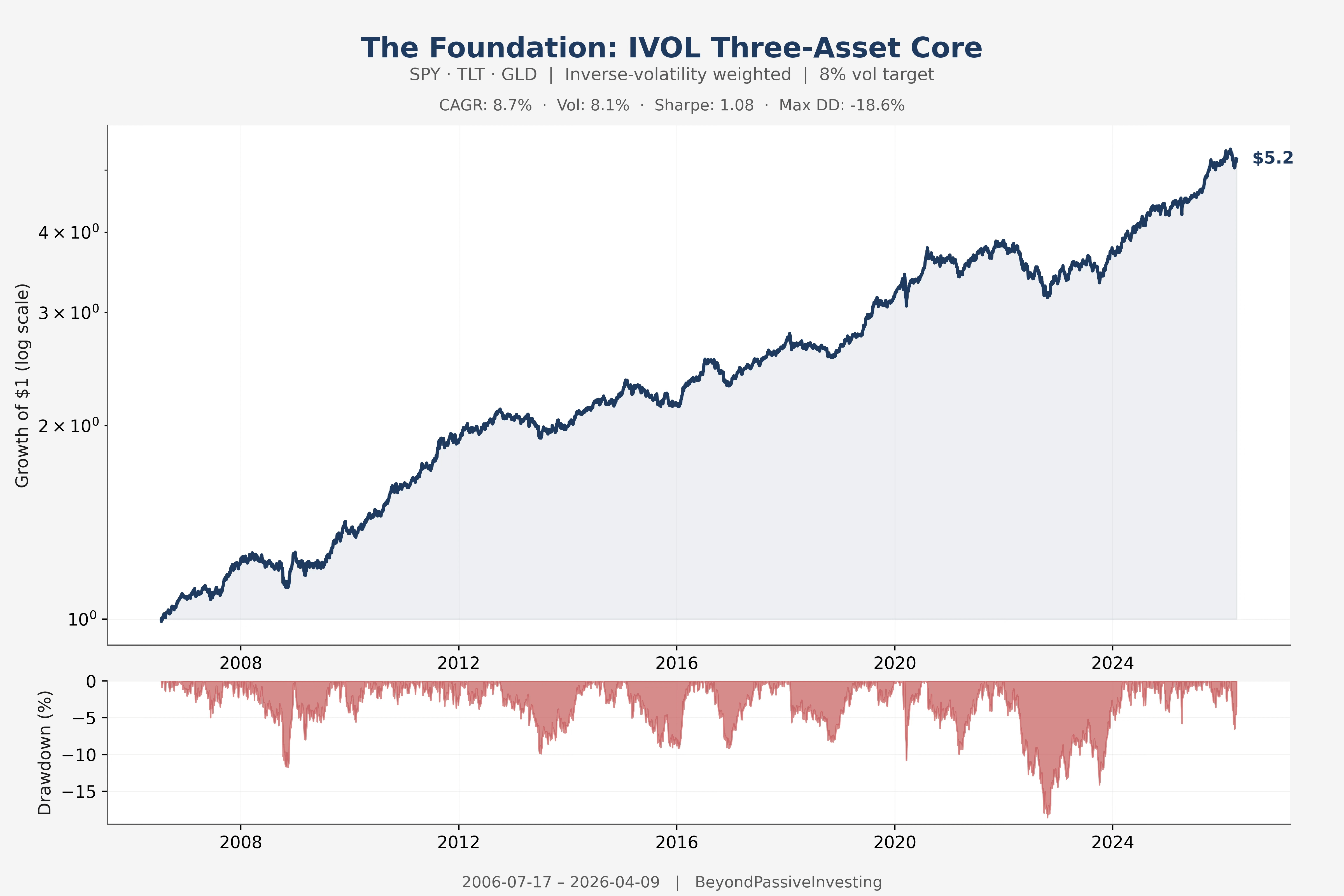
The IVOL three-asset core — SPY, TLT, and GLD weighted by inverse volatility with an 8% portfolio vol target — is the starting point. Everything else in this article is an overlay on top of it.
The Ingredients
Here are all eight seasonal satellites, each shown at full allocation on their active days. The gray line in each panel is the core for reference.
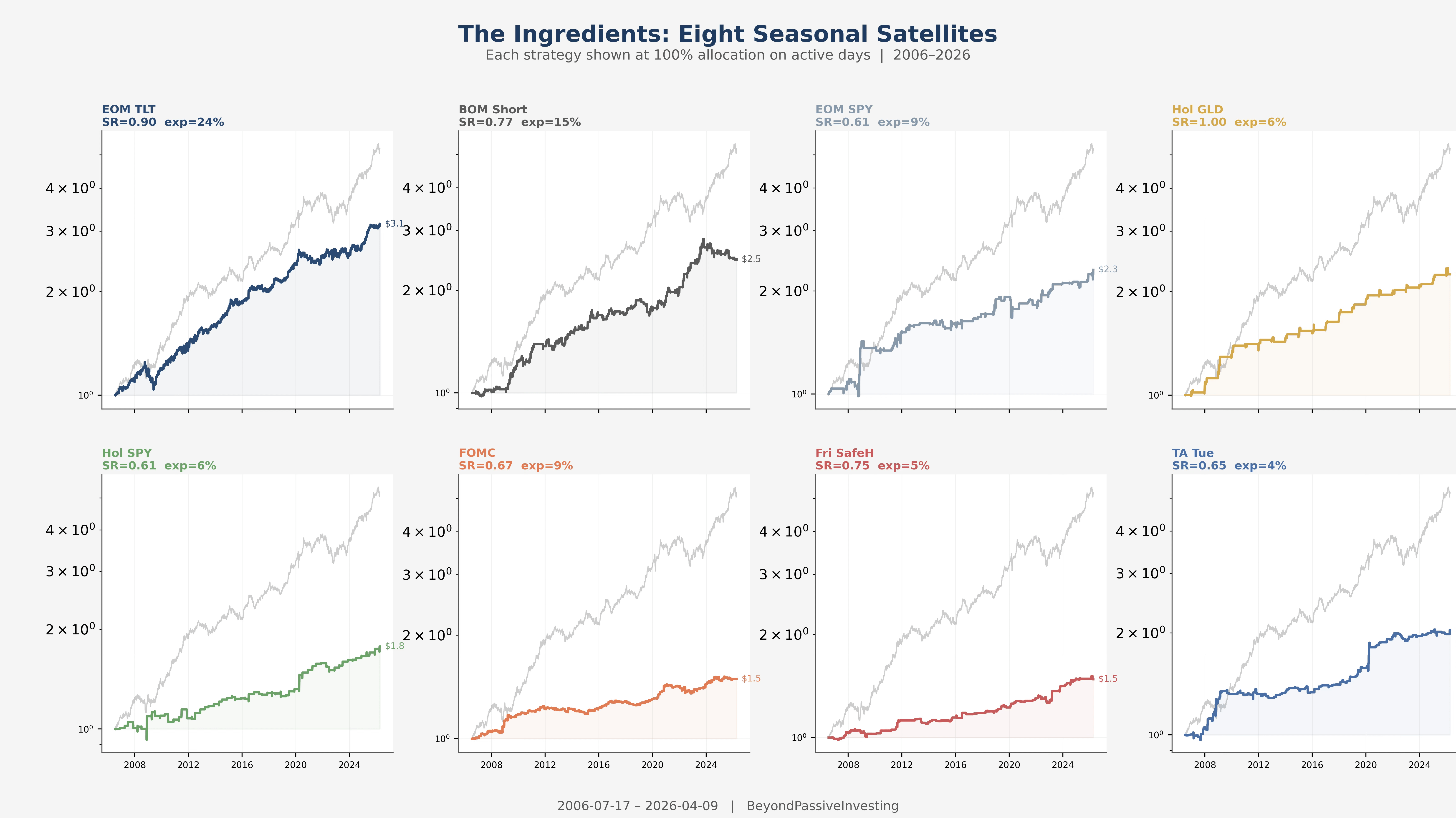
The strategies span a wide range. The end-of-month TLT trade is active on 60 days per year, Turnaround Tuesday on fewer than 10. Some are unconditional calendar effects, others conditioned on VIX regime or stock-bond relative performance. What they share is sparsity: none is active more than a quarter of trading days.
The Naive Stack
The simplest combination: take the core, add each satellite as a 10% overlay when active, done. No optimisation, no regression, no opinions about which is better.
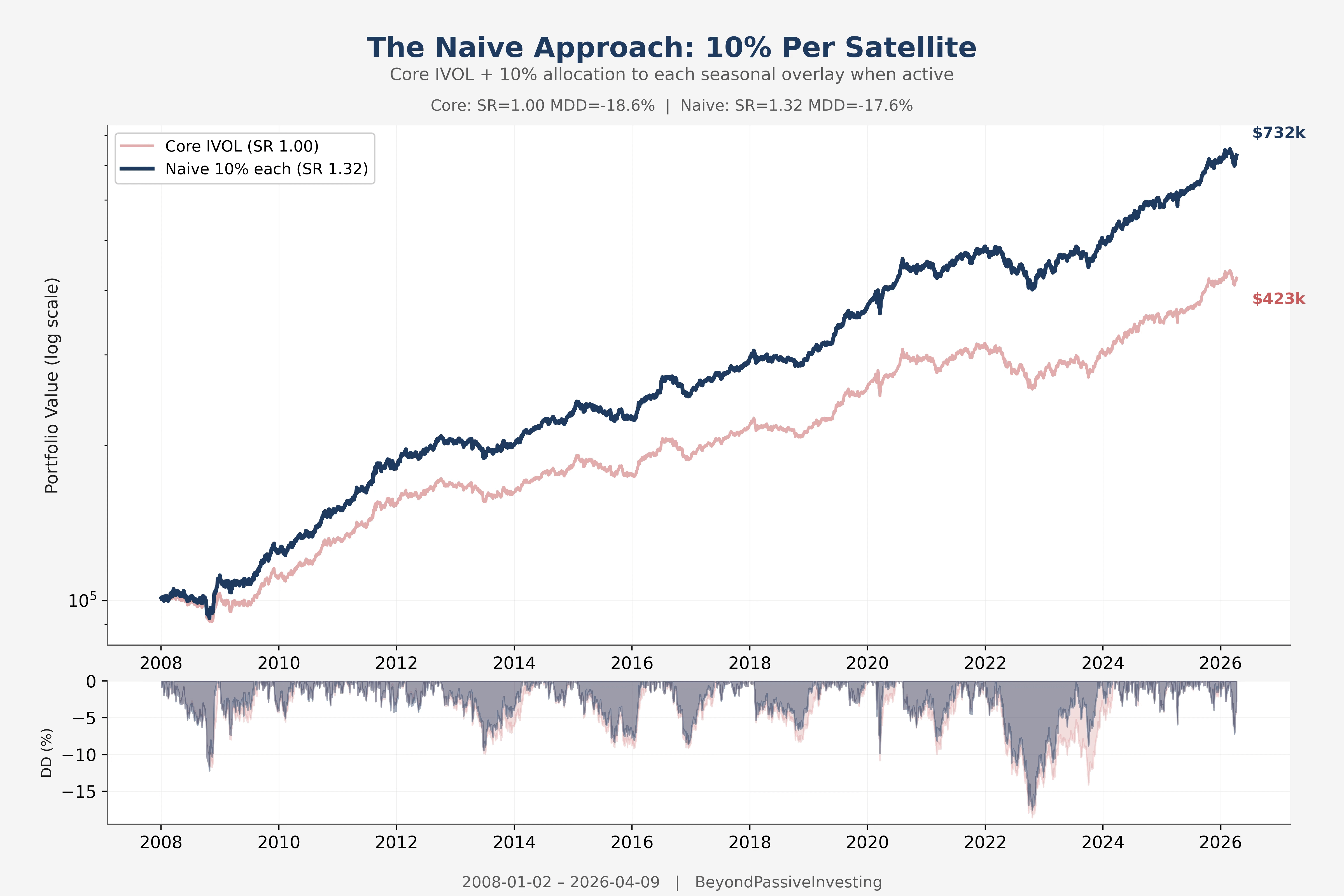
The naive stack takes the Sharpe from 1.01 to 1.31 and turns $100k into $723k. The improvement is real, and it takes zero effort. But equal-weighting is blind — it gives the same 10% to every overlay regardless of whether it adds independent return or just replicates the core.
Why It Works Anyway
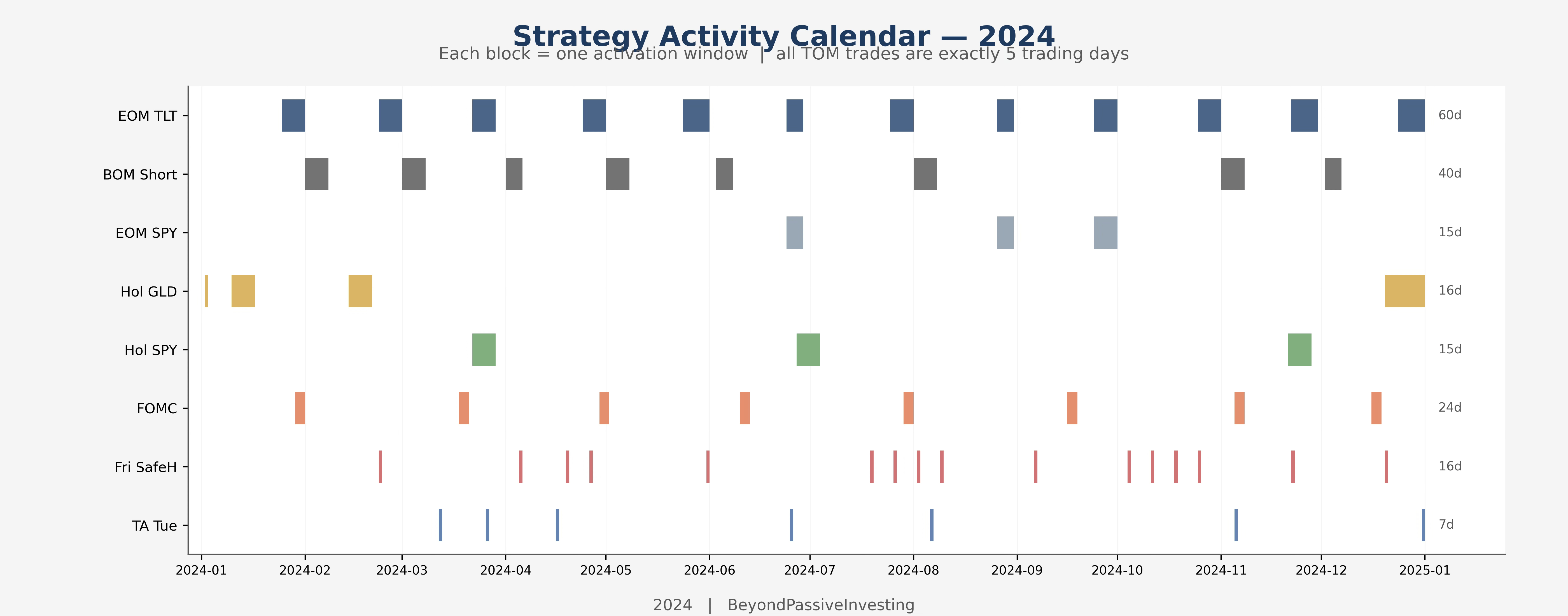
The naive stack works because these strategies are sparse pulses scattered across the calendar. They rarely overlap, so each one contributes returns on days when the others are silent. Diversification here comes not from low correlation but from non-overlapping activation.
The Correlation Trap
The textbook approach to portfolio construction requires a covariance matrix: estimate pairwise correlations, compute the efficient frontier, allocate. That requires hundreds of overlapping observations for every pair. Here, it fails.
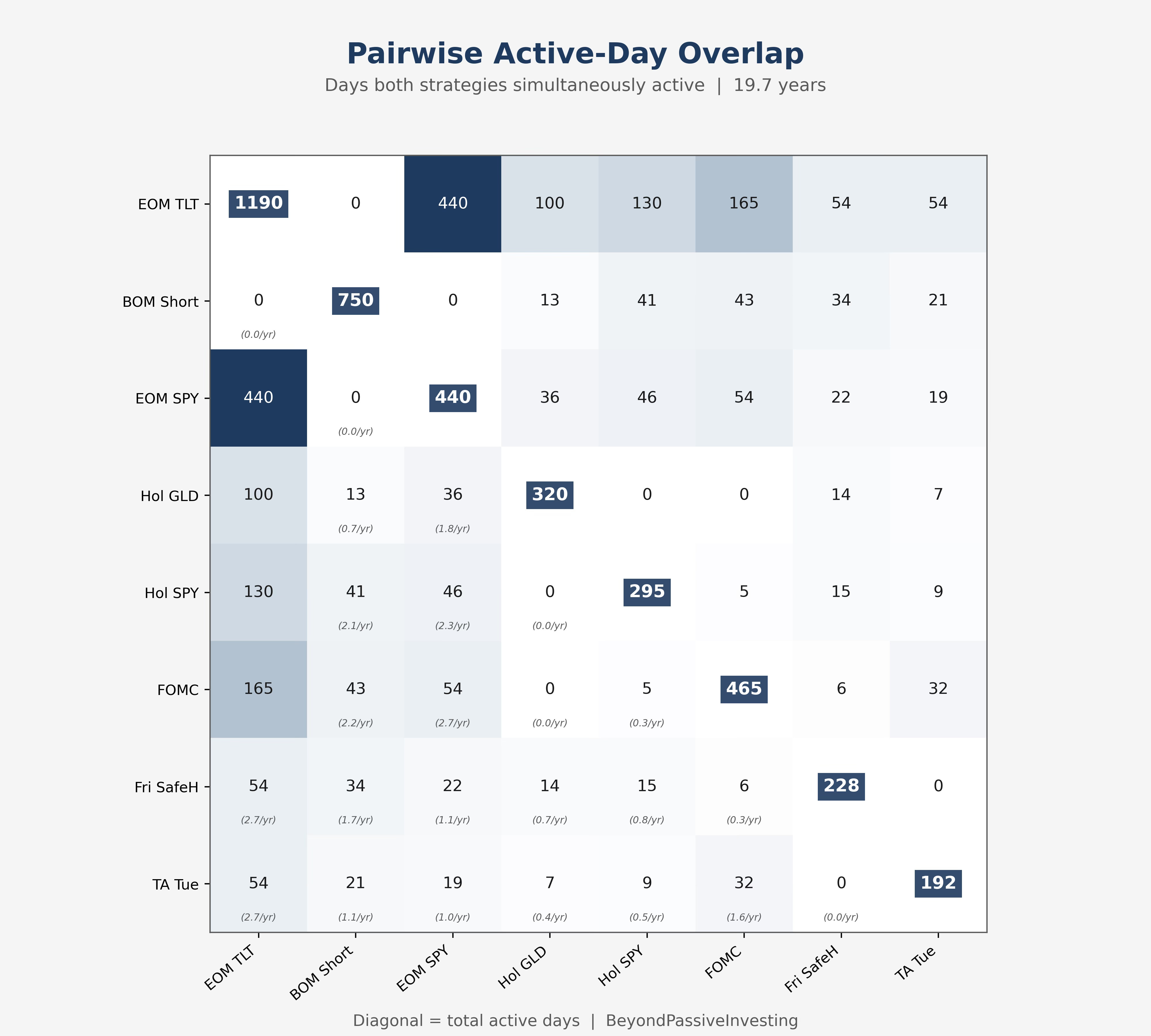
Friday SafeHaven and Turnaround Tuesday share zero active days over 19 years. BOM Short and EOM TLT share zero by construction. Even pairs with some overlap rarely exceed two shared days per year. Any correlation computed from these samples is noise. The covariance matrix is the wrong tool, and more data will not fix it — the sparsity is structural.
Regression: The Right Question
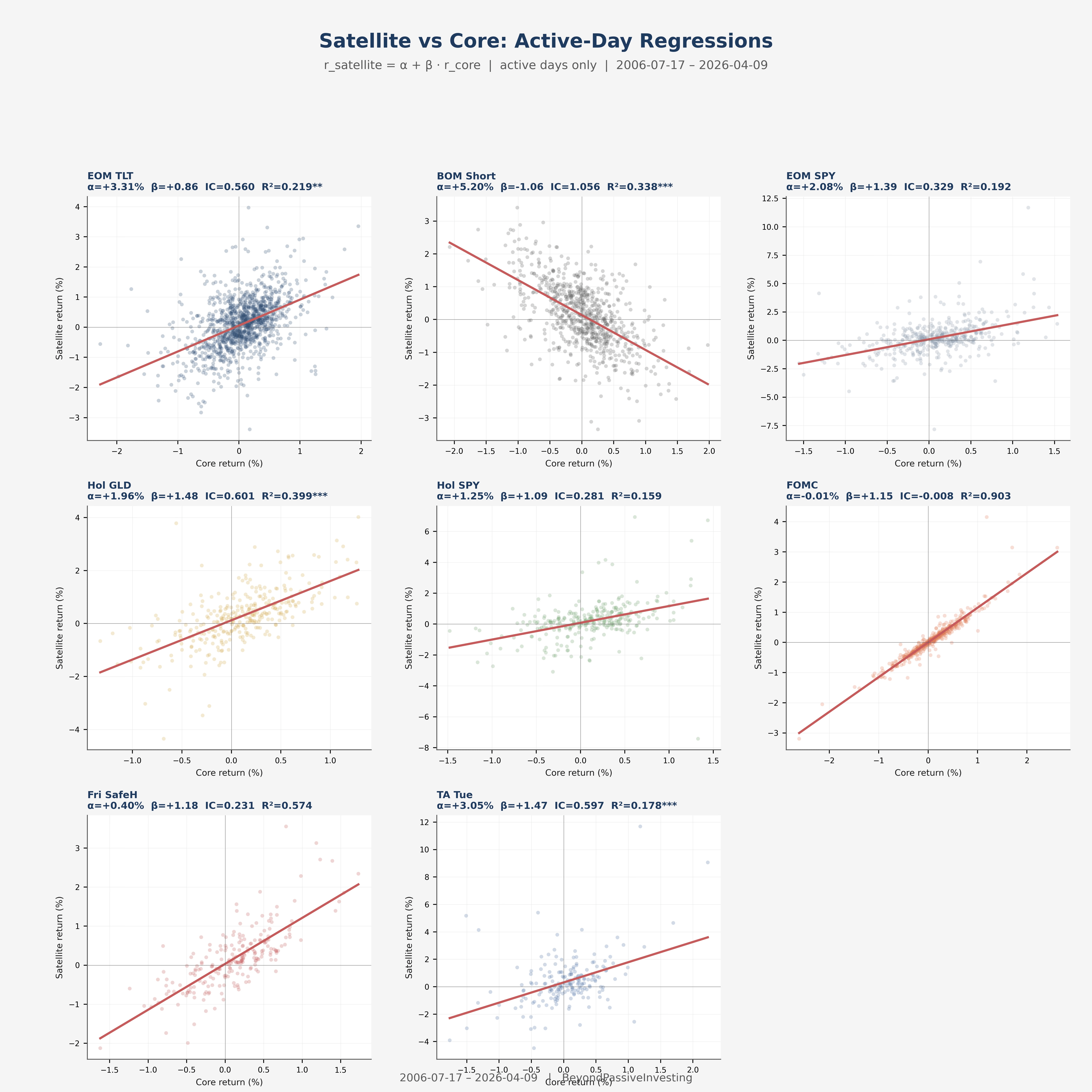
We cannot measure how the satellites relate to each other. But we can measure how each one relates to the core. The core runs every day, so on every active day of any satellite, we have a matching core return. Even the sparsest strategy gives us close to 200 paired observations.
The regression model is straightforward. On the active days of satellite i, we fit:

Three quantities come out of this. Alpha (α) is the intercept — the average return the satellite produces on its active days after stripping out whatever portion moves in lockstep with the core. If alpha is zero, the satellite is just leveraged core exposure dressed up as a separate strategy. If alpha is positive, the satellite generates return that the core cannot explain.
Beta (β) is the slope — how much the satellite moves per unit of core movement. A beta of 1.0 means the satellite tracks the core one-for-one on active days. A beta of −1.0 means it moves inversely. FOMC has a beta of 1.15: on its active days, it behaves like a 115% position in the core. BOM Short has a beta of −1.06: it moves against the core.
Residual volatility (σ_ε) is the standard deviation of what remains after alpha and beta are accounted for. It captures the idiosyncratic risk of the satellite — the part of its variation that has nothing to do with the core. A low residual volatility means the satellite’s returns are tightly explained by core exposure plus a constant alpha. A high residual volatility means something else is driving the returns — noise, or a factor the core does not capture.
The Information Coefficient
The Sharpe ratio of a strategy is its return divided by its volatility. By analogy, the information coefficient (IC) is the strategy’s alpha divided by its residual volatility:

This is the Sharpe ratio of the satellite’s residual returns — the portion that the core cannot explain. A high IC means the satellite delivers consistent alpha per unit of idiosyncratic risk. A low IC means whatever alpha exists is buried in noise. An IC near zero means the satellite is redundant with the core.
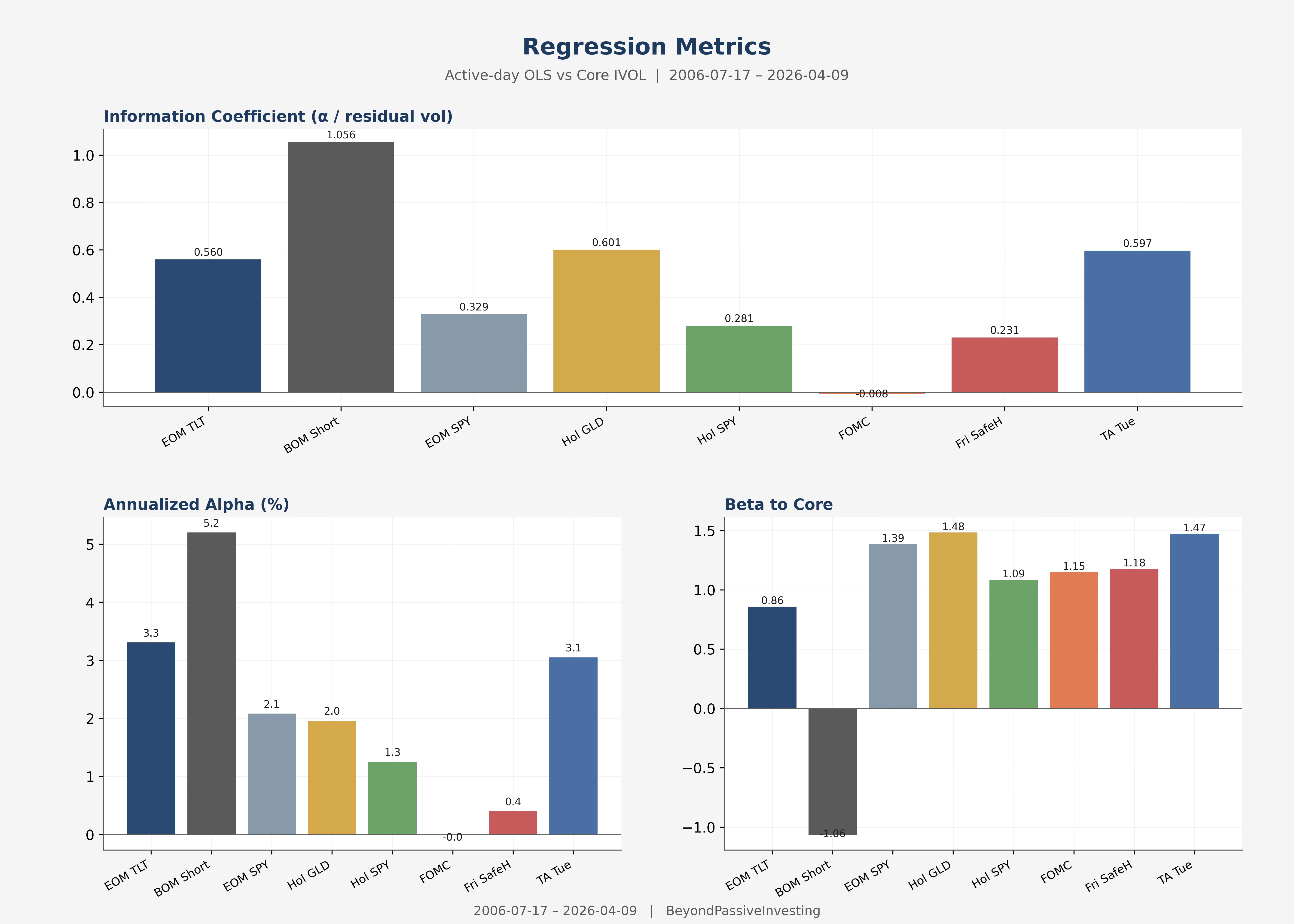
BOM Short dominates with an IC of 1.06 and annualised alpha of 5.2%. Turnaround Tuesday and Holiday GLD follow at 0.6 each. FOMC sits at −0.01: its R² of 0.903 with the core means that on its active days, it is almost entirely explained by core exposure. There is no alpha to allocate to.
That does not make FOMC useless. It is active on roughly 24 days per year that happen to have positive expected return from the pre-announcement drift. Including it at a modest weight is a low-cost way to increase core-like exposure during a favourable window — essentially a form of smart beta. It just should not receive more weight than the prior, because the regression finds no independent edge.
From IC to Weights
The IC gives us a quality ranking. Translating it into weights requires addressing two problems: noisy estimates in early years when the expanding window is short, and the question of how much to trust seasonal effects relative to the core.
Risk premia — the compensation for holding equities, bonds, and commodities through drawdowns — have persisted across centuries. The mechanism is self-reinforcing: risk-averse capital must be compensated, and that compensation does not disappear with arbitrage. Seasonal effects sit lower in the certainty hierarchy. The evidence is real, structural explanations exist, but the mechanisms can erode. A single parameter encodes this gap: belief, set to 0.25. Even when the data strongly supports a seasonal edge, the framework allocates at most a quarter of what it would give to an equivalently-evidenced risk premium.
The weight formula adapts the Treynor-Black framework (1973):
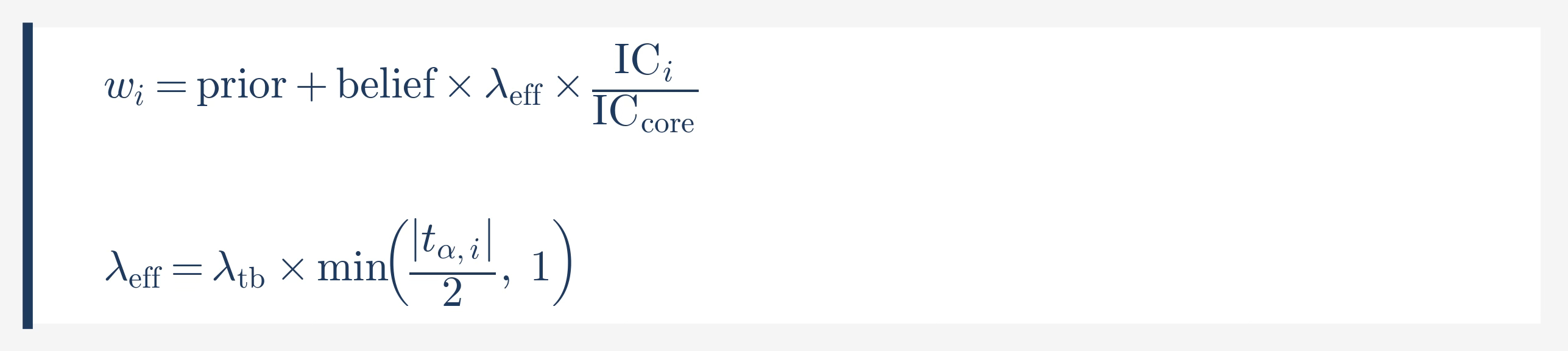
The prior (0.10) is a starting allocation per strategy. The belief (0.25) scales the regression-driven update. And λ_tb (0.70) controls how far the data can move the weight from the prior. The term min(|t_stat|/2, 1) is the confidence gate: it ramps from zero to one as the t-statistic on alpha grows from zero to two. When the expanding window has few observations and significance is low, weights stay near the prior. As evidence accumulates, strategies earn their way up.
This is a Bayesian approach in spirit. Start with a reasonable guess, let the data override it only when the evidence is strong. In practice, it means the early years of the backtest are conservative (weights cluster near 10%), and the later years reflect what the data has actually shown.
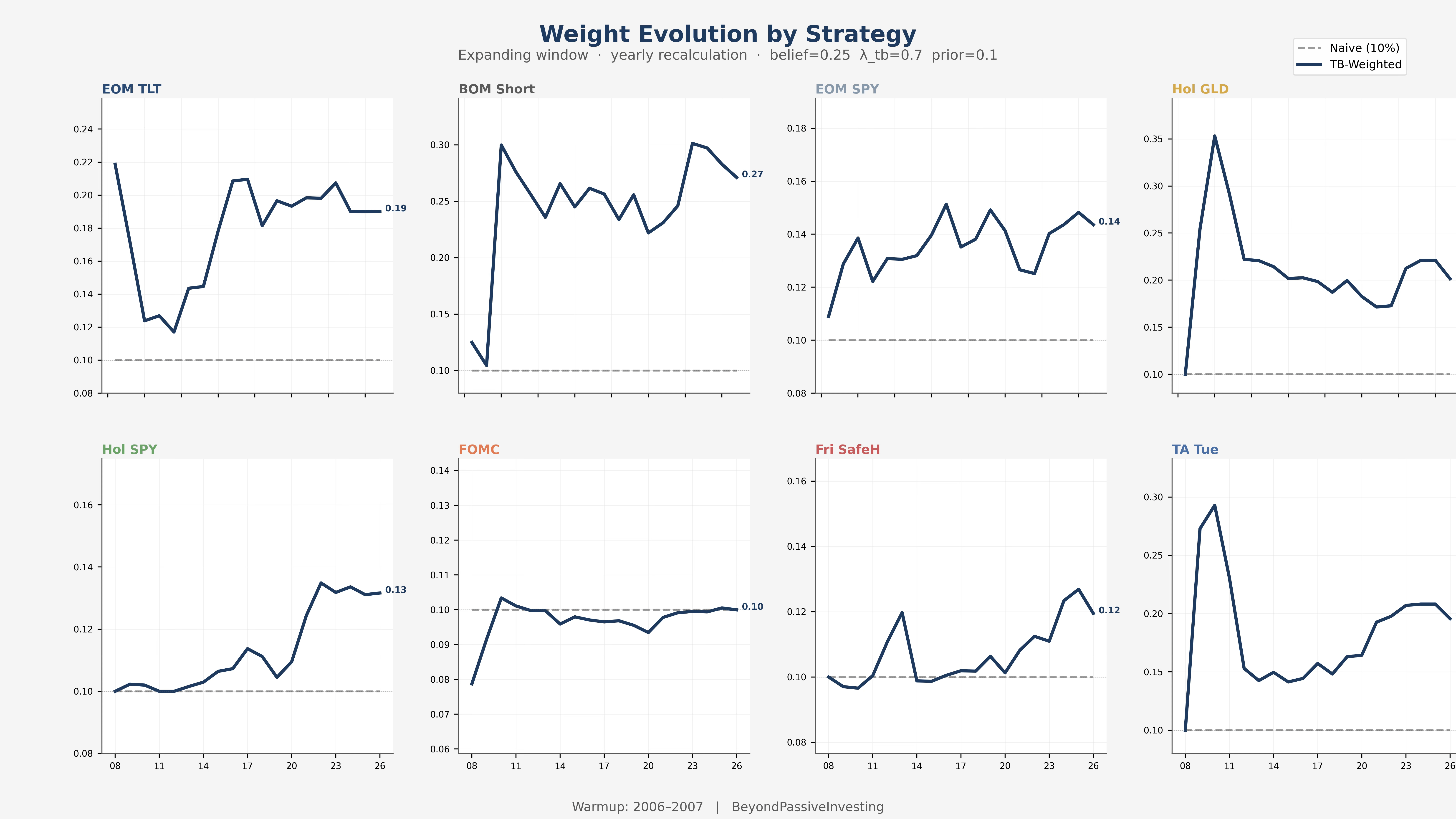
BOM Short starts near the prior in 2008, climbs to 0.27 as evidence accumulates. Turnaround Tuesday spikes early on thin data, then settles as the expanding window dilutes the initial noise. FOMC flatlines at 0.10 for 19 years — the framework finds no alpha and does not allocate beyond the prior.
Acknowledging Tail Behaviour
The regression captures the linear relationship between each satellite and the core. It does not capture what happens in the tails. For most strategies, their losses during core stress are explained by their positive beta. One strategy behaves differently.
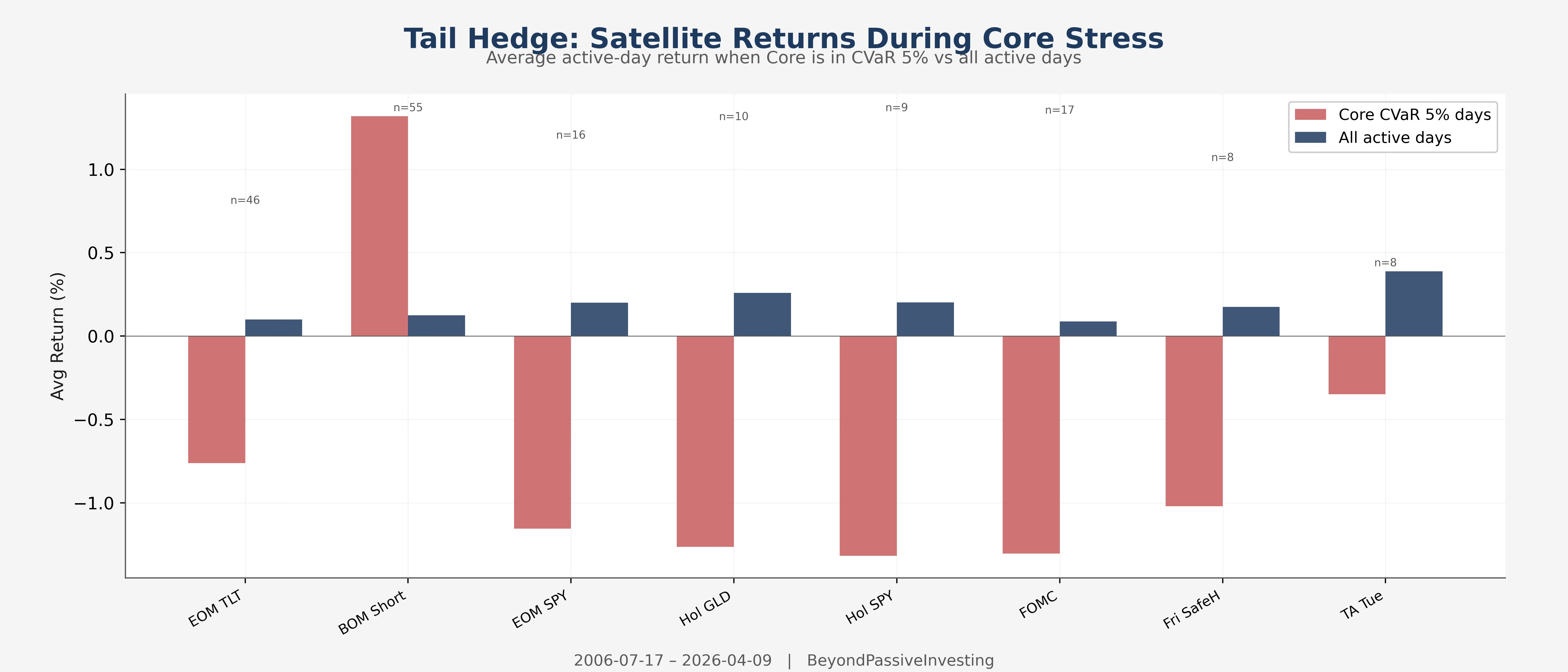
BOM Short averages +1.3% on the 55 days when the core was in CVaR 5% territory. The mechanics are direct: when equities sell off at month-end, bond prices spike, and the short TLT position profits from the subsequent reversion. The portfolio benefits from this beyond what the linear beta captures — large losses in the core coincide with large gains in BOM Short, which compresses the portfolio’s left tail and reduces the drag that extreme drawdowns exert on compound growth.
A small additive term acknowledges this tail behaviour in the weighting:
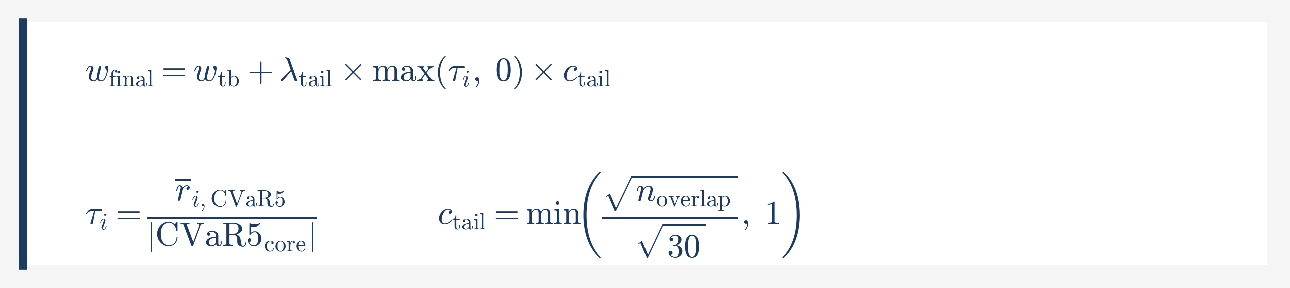
The confidence gate uses 30 observations as threshold because tail events at 5% frequency produce only 0.5–3 observations per year per satellite. Reaching 30 takes 10–15 years of data — below that, the mean tail return estimate is too noisy to act on. The adjustment is positive-only: strategies that lose during stress are already penalised through lower IC in the regression.
With λ_tail at 0.10, BOM Short moves from 0.27 to 0.39. All other strategies stay at their TB weight. The Sharpe improves by 0.05, the maximum drawdown improves from −16.1% to −15.0%. The adjustment is modest, and the more useful takeaway is directional: strategies that profit during portfolio stress are worth actively seeking, because their compounding benefit exceeds what a linear regression can measure.
The Complete Portfolio
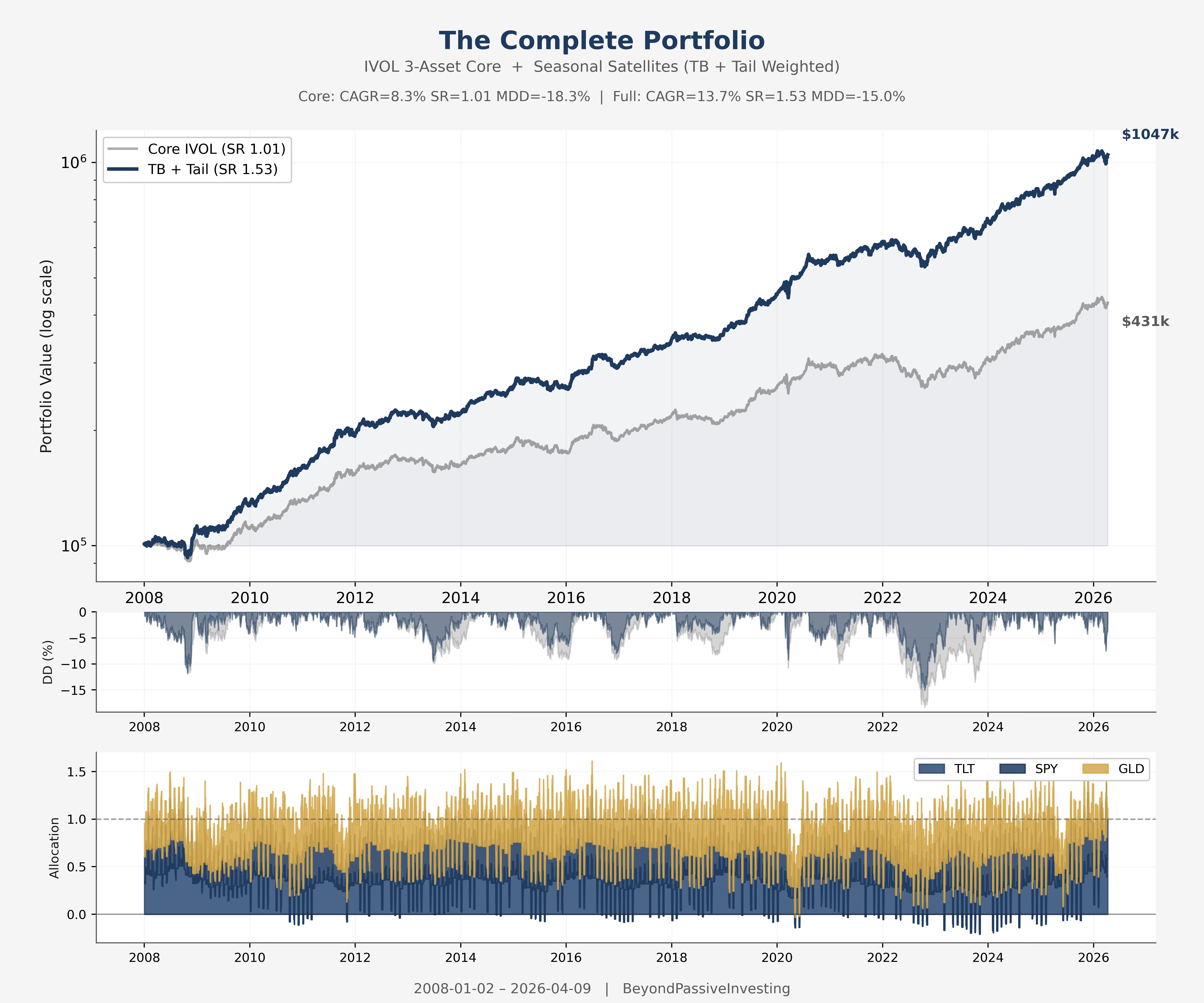

The naive stack captures the diversification of sparse, non-overlapping strategies. The regression separates alpha from beta and identifies which satellites contribute independent return. The Bayesian prior with confidence gating ensures the early years stay conservative and the data earns its influence over time. The tail adjustment modestly rewards the one strategy that protects the portfolio during drawdowns. From core to final portfolio: +0.52 Sharpe and 3 percentage points less maximum drawdown, after all trading costs.
Beyond Passive
Portfolio construction here is not about finding optimal weights. It is about building a framework that makes honest decisions with limited information. Pairwise correlations between strategies that share a handful of overlapping days per year are meaningless. The right question is: what does each strategy add to the portfolio I already have?
Three parameters govern the system: belief (how much seasonal effects deserve relative to risk premia), λ_tb (how far the data can move the weight from the prior), and λ_tail (how much to reward crash protection). None is fitted to the backtest. Each is a judgement set before looking at results. That is what separates a framework from a curve fit.
Thanks for the great post!
Would it be possible to share the notebook for this analysis?
Very insightful. Thanks.
What if you don't have a core system, just hundreds more or less (un)correlated small edges like seasonality, mean reversion, momentum, ... which have the same problem: very small number of trades each, hardly any varition most of the time, some trades of systems in groups of similar systems overlap but some groups do not, especially not between groups? What would the approach be in this case? How would one size positions and construct something else than an equal weight portfolio of these kind of edges? I use equal weight 1/N and depending on N (max open positions) I manage exposure and draw down. Higher N lower drawdown and lower CAGR...